Solving Problems with Inequalities in Two Variables
Student Summary
Suppose we want to find the solution to x−y>5. We can start by graphing the related equation x−y=5.
When identifying the solution region, it is important not to assume that the solution will be above the line because of a “>” symbol or below the line because of a “<” symbol.
Instead, test the points on the line and on either side of the line, and see if they are solutions.
For x−y>5, points on the line and above the line are not solutions to the inequality because the (x,y) pairs make the inequality false. Points that are below the lines are solutions, so we can shade that lower region.
Graphing technology can help us graph the solution to an inequality in two variables.
Many graphing tools allow us to enter inequalities such as x−y>5 and will show the solution region, as shown here.
Some tools, however, may require the inequalities to be in slope-intercept form or another form before displaying the solution region. Be sure to learn how to use the graphing technology available in your classroom.
Although graphing using technology is efficient, we still need to analyze the graph with care. Here are some things to consider:
- The graphing window. If the graphing window is too small, we may not be able to really see the solution region or the boundary line, as shown here.
- The meaning of solution points in the situation. For example, if x and y represent the lengths of two sides of a rectangle, then only positive values of x and y (or points in the first quadrant) make sense in the situation.
Visual / Anchor Chart

Standards
A-REI.124 questions
Graph the solutions to a linear inequality in two variables as a half-plane (excluding the boundary in the case of a strict inequality), and graph the solution set to a system of linear inequalities in two variables as the intersection of the corresponding half-planes.
A-CED.36 questions
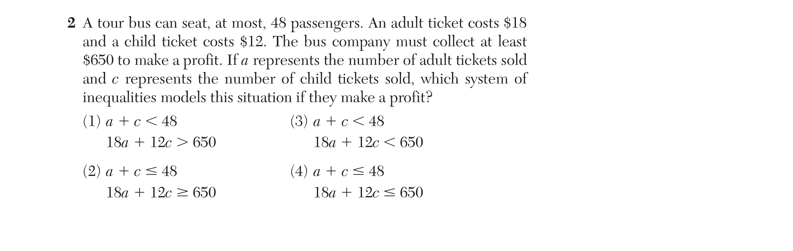
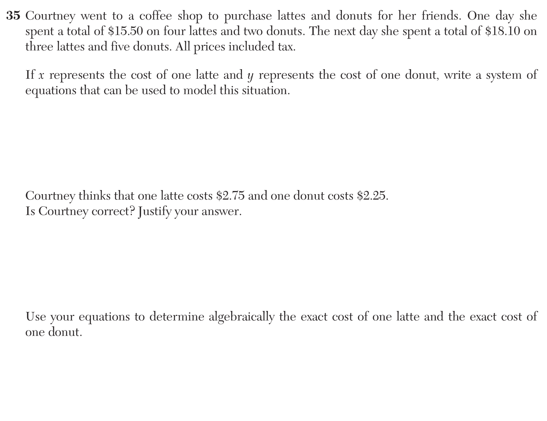
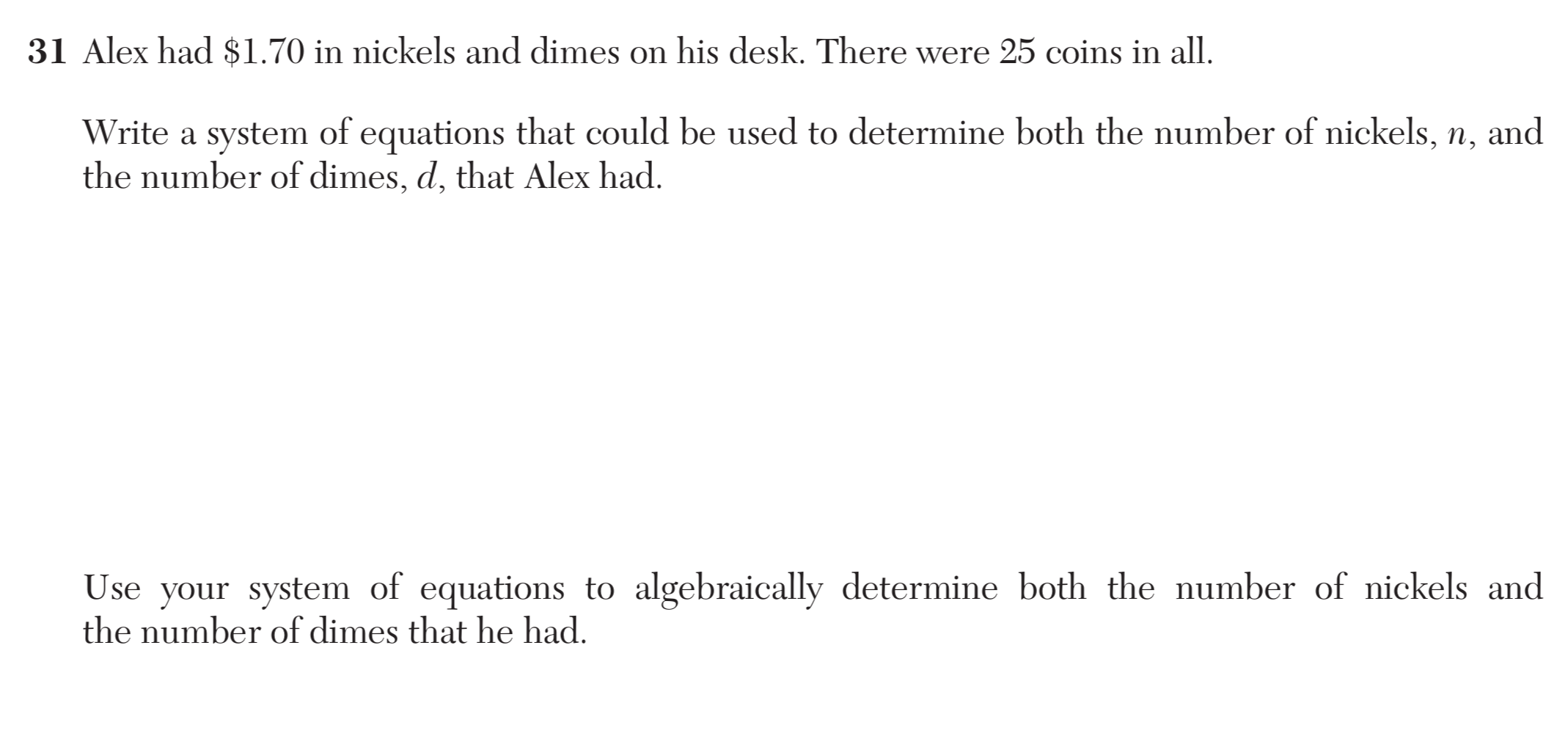
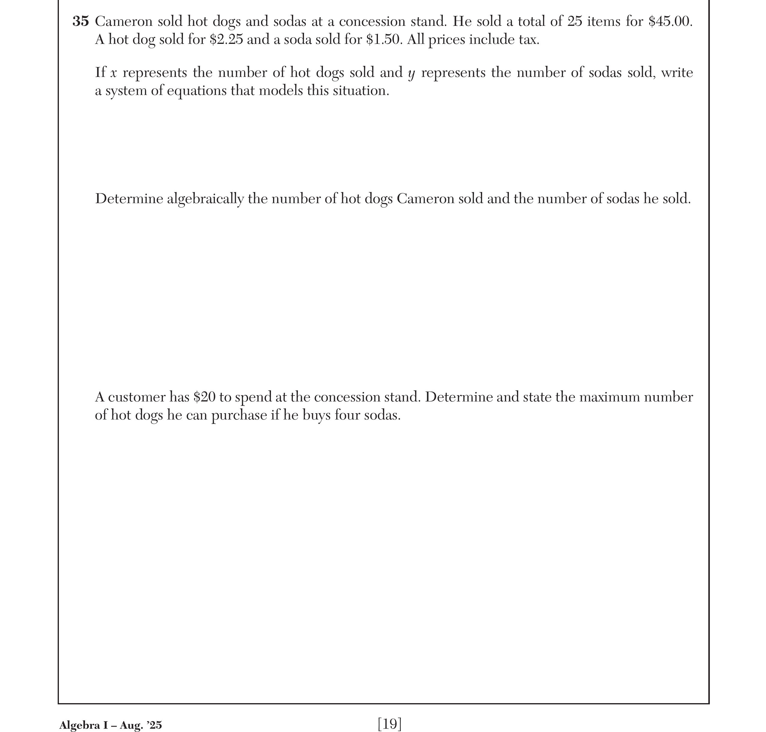
Represent constraints by equations or inequalities, and by systems of equations and/or inequalities, and interpret solutions as viable or non-viable options in a modeling context.